Consistencia del grosor de tejido blando
Visualization and analysis of soft tissue consistency through cones. The size of the cone will be determined by the defined soft tissue study and consist of three regions: in red, soft tissue distances are displayed that are shorter than those that can be accommodated within the soft tissue study, in yellow the data from the study would be above from the mean plus three times the standard deviation and below the mean minus three times the standard deviation. The yellow stripe would accommodate 99.7% of the distribution, according to Chebyshev´s theorem, which assumes a normal distribution of the data. Finally, green is the soft tissue thickness between the mean +- the standard deviation.
The analysis will consist of determining, for each cephalometric landmark, the region of the cone of the corresponding craniometrics landmark in which it is located, or verifying the inconsistency at that point.
 Figure 1. Visualization and analysis of soft tissue consistency through cones with Skeleton-ID in a positive match. For each cephalometric landmark (magenta), the cone region of the homologous craniometrics landmark in which it is located within the defined tissue study is visualized. We can see how, in the green stripe, the soft tissue thickness is between the mean ± the standard deviation (n’ – n, al’ L – al L, al’ R – al R, sn’ – ss, ls’ – pr, li’ – id, pg’ – pg, gn’ – gn). In the yellow stripe, above the mean plus three times the standard deviation (g’ – g) and below the mean minus three times the standard deviation (zy’ L – zy L, zy’ R – zy R, go’ L – go L, go’ R – go R). The pairs en’ – d and ex’ – ec have not been analyzed due to the lack of data in the statistical study.
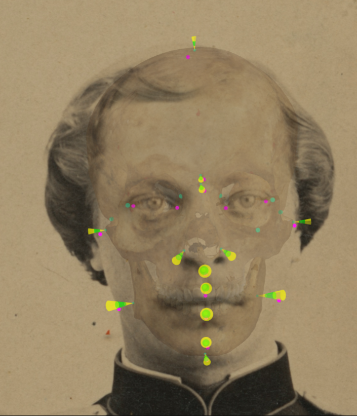 Figure 2. Visualization and analysis of soft tissue consistency through cones with Skeleton-ID in a negative match. For each cephalometric landmark (magenta), the cone region of the homologous craniometrics landmark in which it is located within the defined tissue study is visualized. We can see how, in the green stripe, the soft tissue thickness is between the mean ± the standard deviation (al’ L – al L, al’ R – al R). In the yellow stripe, above the mean plus three times the standard deviation (g’ – g, n’ – n, sn’ – ss, li’ – id, pg’ – pg, gn’ - gn) and out of range (zy’ L – zy L, zy’ R – zy R, go’ L – go L, go´R – go R, ls’ – pr, v’ – v). The pairs en’ – d and ex’ – ec have not been analyzed due to the lack of data in the statistical study.